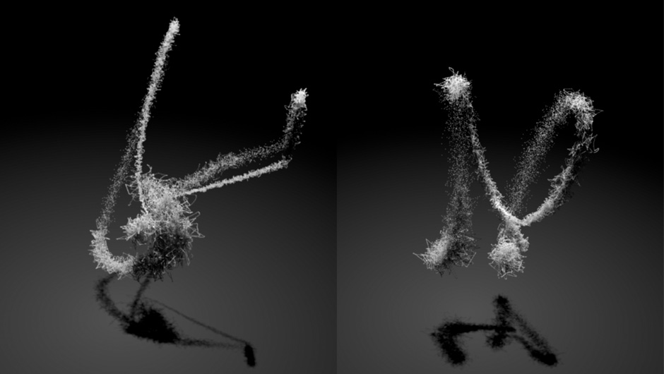
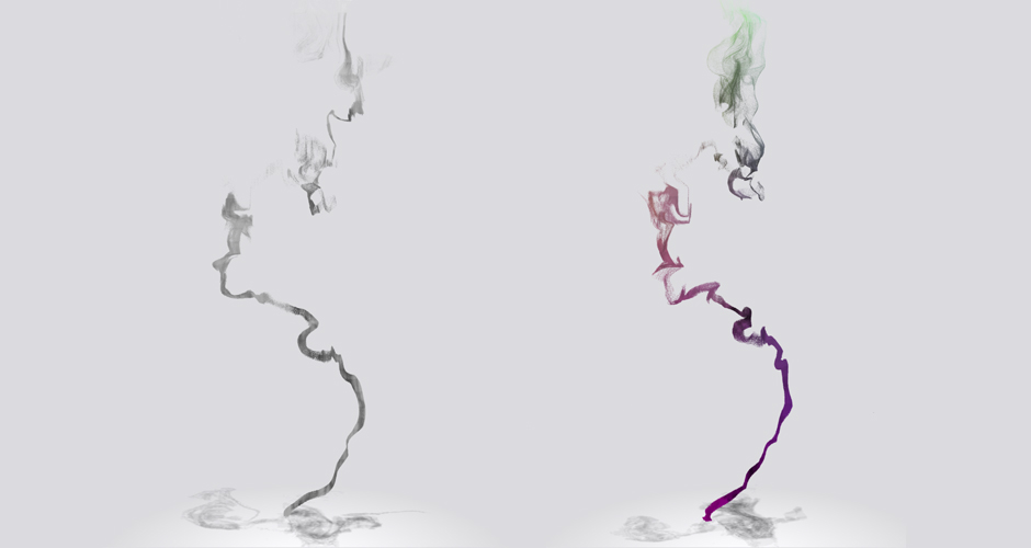
view the high resolution example
view the mid resolution example
view the low resolution example
A good link is a good gift…
When we try to code anything in our studio, the first thing we do is to search for information about the subject in order to find papers and techniques that could help us to develop what we want. The bad thing about it is that you loose a lot of time in Google trying to find that specific paper that reveals the “secrets” of the math behind the code.
But some time thing are even worst, because we do not even know what we are searching for, and this is when a good starting link is a good “gift”. In our case finding this blog has been a perfect starting point to find GPU techniques and papers related to those techniques.
The work made by these guys is amazing, but more important is that they talk about all the methods used in their works, so you can start searching by your own if you like to do something like. In our case we wanted to make some particles animations like the ones found here, and they have the perfect starting point in this post.
Two main things we would have to deal with in order to get a simple particle animation, these are:
- Create a fluid like animation for the particles.
- Shade the particles to give some volumetric effect.
Curl Noise:
In the post from DirectToVideo we found two lines that called our attention, they talked about a technique to fake velocity fields for a procedural fluid flow called “Curl Noise” created by Robert Bridson, and this is how we found this paper. In this paper the author defines a divergence free noise suitable for velocities simulations.
Using divergence free potentials is important for a flow simulation because it avoids sinks in the flow (try to think that with this you will not get all the particles going to a single final position, like a hole in space). Implementing is quite simple because you only have to calculate the differentials of the potentials (noises) used to create your field.
To create the potentials used for the velocities we used the equations from the next image. The only assumption that we made is that every scalar component from the potential vector field is a 2D function that would satisfy the rotor operator.
The second group of equations explains our assumption, we defined each axis potential as a function of the other two axes in order to use 2D textures for the tree potentials, this way we do not need 3d volume textures for each potential. With this assumption we ended with tree 2d textures that defined our potential so the velocity would be defined as the rotor operator applied to the potentials field as you can see in the equations. To calculate the partial derivates we only had to calculate the finite difference the given textures, and the good thing is that since we have our point defined in a texture space we could use this position to get the potential value for the tree defined potentials.
Now that we know how to create the velocity field we needed tree good noise textures to work with, this is an issue because if we load some external textures our development would be tied to those images. So we decided to create the noise textures by ourselves.
Our first approach was to make textures using perlin noise functions, but we then found that they are somehow expensive to calculate so we opted for a more practical solution, simplex noise, and the best thing is that we found one webGL hack here. With the noise functions solved we only needed to make it turbulent, so we found that we could add higher frequencies to get a turbulent noise, you can read a full explanation here.
This is how we ended creating our own textures that we could change in realtime (not in every step), and would allow us to find the best noise suitable for our needs. In the next image you can see the same base noise with a without turbulence.
Saving the potentials as textures add a new problem to solve, textures in webGL only saves 8 bits per channel, so if you naively try to save the potential value in one channel you will only save a 256 units space value. This means that if your noise is defined in the rank [0-1] you will find jumps of 1/256 in your noise. To solve this you can pack your one dimentional value in the RGB components of the textures, this would give you a resolution of 2**24 for a given value.
We use two functions to pack and unpack floating point values in the textures, these are defined like this:
vec4 pack(float value) {
return vec4(floor(value * 256.0)/255.0, floor(fract(value * 256.0) * 256.0)/255.0 , floor(fract(value * 65536.0) * 256.0)/255.0, 1.0);
}
float unpack(vec4 pos) {
return pos[0] * 255.0 / 256.0 + pos[1] * 255.0 / 65536.0 + pos[2] * 255.0 / 16777216.0;
}
The first function wraps one value in RGB components, so you can save one value with very high resolution, the second function unwrap the RGB components to the original value. Note that the function do not save negative values, so is up to the programmer to define how the unwrapped value is going to be treated. The bad news about it is that you need a whole texture to save one value, so if you want to save one 3D position of one texture you will need three textures for it.
The last paragraph defines the main bottleneck of the application, since we have to save the particles positions to run the simulation we need to traverse all the particles three times to save each axe position in a different texture. In the next image you can see one of the axis aligned position textures used.
Particles shading:
To shade the particles we applied the same technique from our previous posts (http://www.miaumiau.cat/2011/06/shadow-particles-part-ii-optimizations/), but we modified it to accept a variable bucket quantity so we could adapt the final resolution of the shadows in the volume. Since we can set many more slices we saw that the interpolation used between two slices was not necessary, so we took it away to get some more speed.
Now that we can change the buckets count we had to look for the best compromise among the buckets size, the quality of the shadows volume, and the quality of the floors shadow, for a 2048 texture size we found that the initial 8×8 buckets count is a very good compromise for the given parameters. With this in mind if you want to implement good quality shadows in your volume we recommend 16X16 buckets slices, but the final shadow for the floor will be very slow. In the next image you can see one test of the shadows with and without color.
The process:
With the curl noise, the volume shadows and the floating point issues solved we ended with an algorithm of seven steps, this process requires five render targets changes and we need to traverse all the particles five times. Three times to save the particle´s current position, one for the shadows and one final to paint them all.
We also perform some window, or 2D, calculations over the fragment shader to get the correct blurring for the final composition, we also calculate the potentials using the fragment shader.
Two things should be implemented to get a correct particle´s rendering, first of all, if we want to render all the particles we will need to use blending, but this requires that all the particles get to be sorted (if not you will se much less particles than the ones you expect). The other thing is to use another texture to control the life of the particle. This way we don´t have to reposition the particle in the emitter every time it reached it´s “y” limit.
Some workarounds:
The previous commented process have a huge bottleneck saving all the particles positions, so we wanted something faster to get the particles position. So instead of calculating the positions in a step way, we defined the positions based on a path (a Bezier path), this Bezier would be affected by the noise so we only would need one texture to save the Bezier points.
One good thing about using a Bezier path is that you can use the linear interpolation of the textures to get the current particle position in the curve, this way we don´t have to save all the particles positions, instead we only have to save some Bezier points in a texture (to be concrete 512 points) and then we read the particles positions using the gl.LINEAR function to calculate the point interpolation from the texture reading (all of this for free).
So if you can have as many paths as the height of your texture, and each path can have as many points as the width of the texture. In our case we only used to paths, you can see some images of the implementation.
The previous image shows the positions texture using two paths, and the 3D result of the Bezier applying the curl noise. This way we don´t need to save the positions in three textures. The bad thing about it is that all the particles are constrained to the Bezier path, so we cannot perform some particles dispersion.
Instead of applying the curl noise to the Bezier path we could use some of the total particles to create a volumetric path, and use some more to make some particles dispersion with the first technique. In the next image you can see how the Bezier paths are rendered using just one texture.


100K Particles self-shaded from miaumiau interactive studio on Vimeo.
So if we use the Bezier path to move some initial particles, and we also move the emitter position over the path, and we finally define the exit initial velocity for the dispersion particles in the emitter using the bezier´s tangent, we think we could make something like this, but with much less particles 🙁


