
Shading particles can be frustrating sometimes, there’s a lot of geometry and the particles tend to look flat when working with direct lighting effects and shadows since they don’t account for the volumetric effects of the particles.
The previous issue have been solved using different techniques that are used to shade particles such as volume shadows (displayed in the next image), which is pretty nice to simulate scattering effects over the particles, but these methods do not solve global illumination effects that provide better information of the particles as a whole.
Particles Volume Shadows From Nvidia
In that regard Global illumination can be solved for particles pretty neatly using voxel cone tracing, this method is pretty useful since it provides a method to calculate the ambient occlusion and emissive effects over the particles. Soft shadows can also be evaluated using the same structure generated for the cone tracing.
The original idea comes from Edan Kwan who used this technique to render the moon particles of his Lusion site, among other projects. The particles approach for Voxel Cone Tracing is based on a simplification done when dealing with the voxelization.
Voxel cone tracing has the limitation that the geometry requires to be voxelized every single frame, which can be expensive in terms of performance, but particles can be treated as single points allocated on each voxel; this simplifies the voxelization process to a single draw call that scatters all the particles inside the voxel structure.
Voxelization can be done firing one draw call that positions each particle on the corresponding voxel using the vertex shader to reallocate (scatter) each vertex (point) inside a 2d texture that simulates a 3d texture. This process allows to allocate particles as big (or small) as the segmentation of the space (each voxel.).
The idea is to treat the render target as a “sprite sheet” of slices from a 3d texture, the texture is layered into different depth slices that correspond to a different depth layer from a real 3d texture, this way the renderer can allocate all the particles in their corresponding voxels using a single draw call. The following image shows the result of the voxelization step and layering.
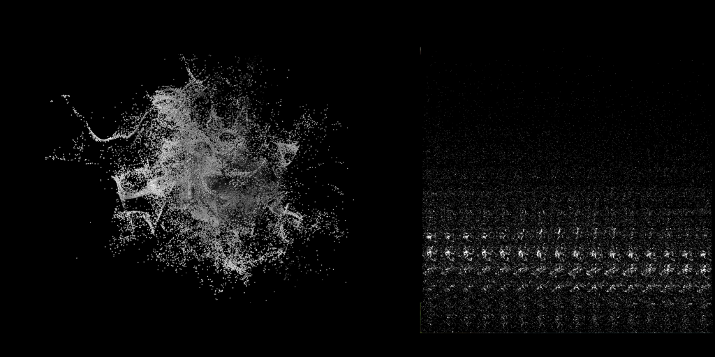
Particles are rendered in different depth layers into a 2D texture like spritesheets
When the representation of the particle is bigger than a voxel, like big spheres, the voxelization can be simulated instancing the particle itself, the idea is that each instance represents the surrounding of the voxel from the original particle, updating the voxels inside the cube defined by the bounding box of the particle’s representation. The occlusion value can be diminished based on the distance from the instance to the center position of the particle, which is useful to simulate partial coverage of the voxel, and the emission value can be the same one for each of the voxels enabled for the corresponding vertex.
Once the particles are allocated the next step is to calculate the mip mapping of the texture, this step can be challenging since the previous step rendered the particles inside a 2D render target, this implies that the data has to be passed from the 2D texture to the 3D one. This is required since the Voxel Cone Tracing algorithm works with linear filtering over the mipmaps from a 3D texture.
Three.js webGLRenderer allows setting the render target to render the data to each layer of a 3d texture, which is really useful to reallocate the data; sadly it implies firing too many draw calls which depends on the depth dimension of the 3d texture.
This process can be improved by doing things “manually” meaning that the step can be done using vanilla WebGL, which allows to setup a shader that defines up to four output layouts, this can reduce the amount of draw calls to update the 3d texture.
Once the data is allocated into the 3d texture the next step is to calculate the mipmapping, which WebGL allows to make it using the API, there’s no need to setup a particular shader pass to evaluate it like in WebGPU, the latter requires to create a custom compute shader to generate the mipmapping of the 3d texture.
Having the 3d texture ready is just half of the process for shading, the most important part happens in the shader used to render the particles. Shading requires to traverse the 3d texture using cone tracing (the original paper can be found here), but things are a little different as with regular geometry.
The voxel cone tracing algorithm uses different directions from the normal of the point to shade in order to evaluate the incoming radiance from the whole hemisphere surrounding the point; usually 5 to 9 directions are used to evaluate the lighting arriving to the surface. This can be seen in the following image.
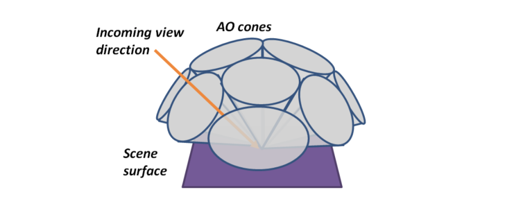
Voxel Cone Tracing uses different cones to gather the incoming light from the hemisphere covering the sample to shade.
For particles, light can come from any direction, which makes normals not so useful, in this case lighting information can be traced from the six main axis orientations, traversing the 3d texture using a cone with a wide open angle to gather as much light data from the corresponding axis, the opening angle can be setup to 90 degrees to connect each cone on the adjacent directions.
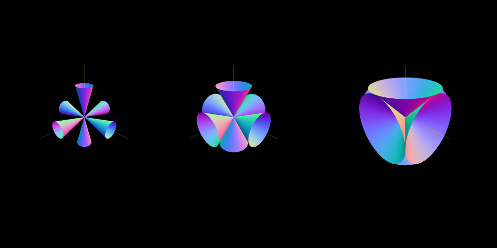
Cone directions used to get the incoming light for each particle, different aperture angles are displayed. Big aperture values cover the total light received on any direction.
Once directions are defined the process is similar as shading regular geometry, the 3d texture is traversed using cone tracing on each direction and the end result is the average of all the directions. Shading can provide very convincing results, but there are some caveats that need to be managed, these are:
– Particles need to be confined into a space in order to voxelize it using a grid: this requires to setup a simulation space big enough to allow the particles to move freely inside the voxelized space. This could be solved with hashing though.
– The voxelization size can affect performance when traversing the 3d texture, luckily global illumination can be thought as a low frequency effect, meaning that there should not be too many hard changes in the ambient occlusion or lighting effects over the space, this allows to use small size segmentations (low resolution 3d texture).
On the flip side using a small segmentation means that many particles can fall into the same voxel, and the rendering of the particles might only update the voxels without taking into account the density information of the corresponding voxel, meaning that it does not take care how many particles are inside each voxel.
This can be mitigated using additive blending when rendering the particles inside the 2d texture, this way the amount of particles is taken into account making voxels reflect particle density with the emission and the occlusion.
The idea is that the RGB channels of the voxels are used to define the emission value of each particle’s contribution inside the voxel, and the alpha channel is used to define the occlusion. Additive blending will increate the RGB value linearly depending on the amount of particles that emit light, and the alpha channel defines the total density (amount of particles allocated in the voxel). Higher density values will contribute to a higher occlusion effect in that region.
– There’s an inherit flickering effect that comes from the voxel cone tracing itself, it tends to happen when particles travel from one voxel to another one, you can overcome this issue increasing the voxeling resolution at the expense of performance, or make a 3d blur pass over the 2d texture smoothing possible flickering effects when transitions happen. Temporal reprojection can also be helpful to mitigate this issue.
Bonus feature… Raytracing
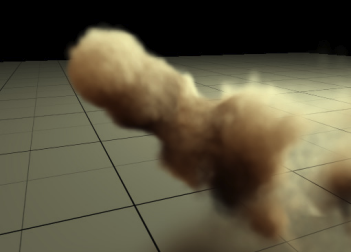
The voxelization step also provides an excellent opportunity to generate an acceleration structure based on the 3d texture generation, which is useful to make raytracing effects like the now show in the next image.
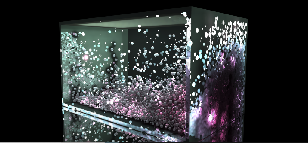
Raytracing can be implemented using an acceleration structure generated when generating the Voxelization
The idea is fairly simple, the scattering shader can be used to save the indices of the particles inside each voxel. In WebGL this can be done saving the indices inside each channel of a fragment, allowing to save up to 4 particles per voxel, in WebGPU this can be done creating a storage buffer that preallocate positions for a predefined amount of expected particles per voxel.
In WebGPU the scattering process and the grid generation can be done using a compute shader, WebGL requires to make up to four draw calls for all the particles to use Harada’s sorting technique to save the indices of the particles
Once the indices are saved the 3d texture can be traversed using the 3DDDA (3d differential discrete analyser) algorithm which allows to traverse the voxels in a optimal conservative way for a given direction. On each step the algorithm checks if there are indices saved for the corresponding voxel and a sphere-ray collision is evaluated for each index, the shading for collision point can be done using the voxel cone tracing.
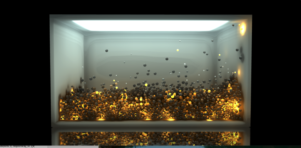
Particles can be rendered using the forward renderer and then use the ray tracing to make specular reflections (shown in the next image), refractions effects or anything you can come up with. Performance wise it’s has the penalties of evaluating the sphere-ray collision for each vertex allocated on each voxel, but the process can limit the amount of voxels to evaluate depending on the distance traversed from the origin of the ray, this is useful to avoid checking reflections or refraction responses from far away objects which might not provide a big contribution to the final result.
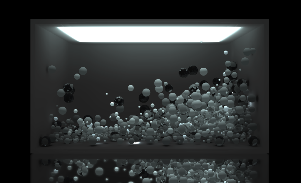
The black spheres display specular reflections raytracing the acceleration structure
Comments
One response to “Indirect Lighting on Particles in Real Time”
Incredible work. I don’t understand anything, but it’s very interesting. The balloons fly beautifully.